Melbourne house pricing

Buying a House in Melbourne: How Much Money Do You Really Need?

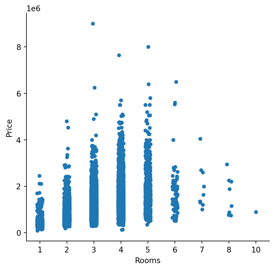
Buying a home in Melbourne feels less like a plan and more like a challenge.

Introduction

Prices keep climbing, choices feel tighter, and suddenly a simple two-bedroom unit sounds ambitious. This raises a practical question: can reading the market actually give buyers an edge?

Motivation

The first thing that came to mind was to focus on what actually drives price differences. In Melbourne, postcode and number of rooms immediately stand out as two key factors. Using Python to analyse the data, this study examines how prices vary across locations and room counts, turning an initial intuition into a structured comparison.

1. Rooms vs Price
2. Postcode vs Price

Rooms vs Price

import pandas as pd
import seaborn as sns
import matplotlib.pyplot as plt
import plotly.express as px
df= pd.read_csv("../../../../data/melb_data.csv")
sns.catplot(df,x="Rooms",y="Price")

_wow it’s a little bit hard to read the graph right? Let’s try to use bar graph.

sns.catplot(df,x="Rooms",y="Price",kind="box")

Bar graph shows how property prices change with the number of rooms. Overall, homes with more rooms tend to have higher prices, which suggests that space does matter. However, this relationship is not perfectly smooth. Prices vary widely for properties with the same number of rooms, especially between three and five rooms, where both relatively affordable and very expensive properties coexist. Interestingly, properties with ten rooms appear to have a lower median price than some homes with fewer rooms. This does not mean that having more rooms makes a property cheaper. Instead, this result is likely driven by the small number of such properties in the dataset and their atypical nature. Homes with extremely high room counts are uncommon and may differ from standard residential properties. For example, they may be located further from central areas or represent older or subdivided buildings. As a result, their prices are not directly comparable to more typical homes. Overall, this figure suggests that while the number of rooms is related to price, it cannot explain price differences on its own. Other factors, particularly location, are likely to play an important role.

sns.relplot(df,x="Rooms",y="Price",kind="line")

The graph reveals that the relationship between rooms and price has limits. Additional rooms raise prices early on, but beyond a certain size, the market becomes far less consistent.

Postcode vs Price

Location matters, but streets are messy. Prices can change within a few blocks. Looking at prices street by street quickly becomes overwhelming. Postcodes offer a cleaner way to group properties, turning scattered price points into patterns that are easier to compare and interpret.

top_postcodes = df["Postcode"].value_counts().head(10).index
df_top = df[df["Postcode"].isin(top_postcodes)]
plt.figure(figsize=(10,5))
sns.boxplot(df, x="Postcode", y="Price")
plt.title("Property Prices by Postcode")
plt.xticks(rotation=90)
plt.show()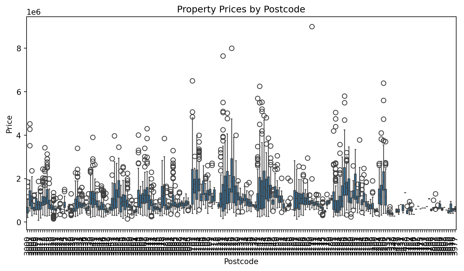

This graph is terrible! When all postcodes are plotted together, the resulting graph becomes cluttered and hard to read. To make the comparison meaningful, only the top ten postcodes by data availability are selected, and median prices are used. Why use the median rather than the mean? Because a few very expensive properties can disproportionately influence average prices.

order = (
    df_top.groupby("Postcode")["Price"]
    .median()
    .sort_values()
    .index
)

plt.figure(figsize=(10,5))
sns.boxplot(data=df_top, x="Postcode", y="Price", order=order)
plt.title("Property Prices by Postcode (Sorted by Median Price)")
plt.tight_layout()
plt.show()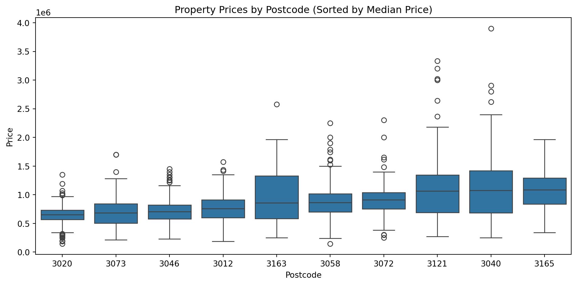

_{Finally… 😮‍💨} Looking at the box plot, it becomes clear that property prices differ quite a lot across postcodes. Some postcodes, such as 3020, 3073, 3046, and 3012, tend to cluster at the lower end of the price range, suggesting that properties in these areas are generally more affordable. In contrast, postcodes like 3121, 3040, and 3165 show noticeably higher median prices, indicating that the typical property in these areas is much more expensive. What is also interesting is that price differences do not only exist between postcodes, but within them as well. Several postcodes, including 3163 and 3058, display wide price ranges, meaning that properties in the same postcode can still vary significantly in value. This suggests that while postcode is a strong indicator of price, it does not tell the full story on its own. Overall, the figure shows that location plays an important role in shaping property prices, but substantial variation remains even at the postcode level, pointing to the influence of other factors beyond location.